| Up: |
|
A Fast and Accurate Light Reflection Model |
| Previous: |
|
The Fully-Assembled Reflection Model |
| Next: |
|
Conclusions |
The distribution function D does not always converge quickly, as illustrated below. The outer curve is the fully-converged solution.
Figure 17: Interactive display of convergence of distribution function D
For certain parameter settings, approximating the infinite summation in D to within 1% may require a few hundred terms. We would therefore like to find a faster way to approximate the sum.
We can write the infinite summation in D as a function of two variables as follows:
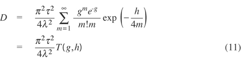
The function T(g,h) is shown in Figure 18 as a function of g, for several values of h.
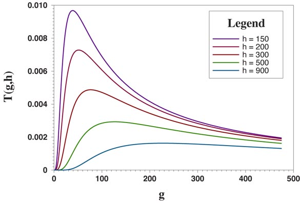
Figure 18: The function T(g,h)
The function T(g,h) can be precomputed and stored in a two-dimensional look-up table. The table can then be used for any combination of geometric and physical parameters.
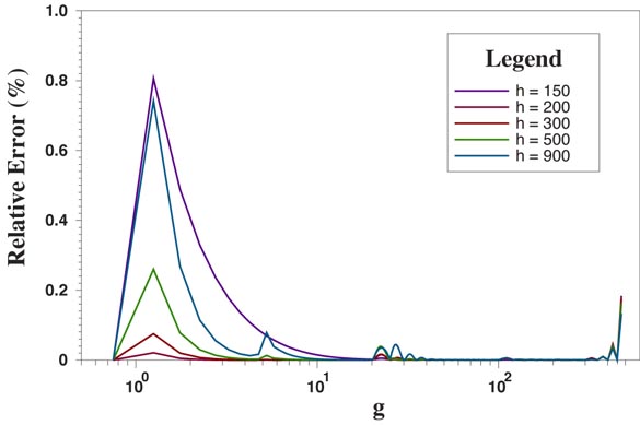
One way of approximating T is with a natural spline surface [PRESS88], which interpolates between given control points, with specified first derivatives at the boundaries. Because T changes rapidly near the origin in the (g,h) plane and is smooth in other regions, we use a nonuniform grid of control points with more points near the origin. At each control point, we evaluate the actual function T; we estimate the boundary first derivatives using a finite difference method. By using a grid of 80×80 control points, we can smoothly approximate the function T. The associated reflectance distributions are therefore smooth. The spline approximation and the exact representation of T essentially coincide in Figure 18. The relative error in T between control points is displayed in Figure 19, and is always less than 1%.
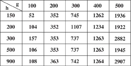
To use the precomputed look-up table for the calculation of BRDF's, we first compute the two intermediate variables g and h from Equations (6) and (9). Because the natural spline formulation uses basis functions of finite extent, we compute a value for T(g,h) by looking at the four control points surrounding (g,h). Table 1 shows the speedup ratio obtained by using the spline approach to compute T to within 1% precision, as compared to evaluating the summation directly to 1% precision, for various values of g and h. The average speedup ratio is about 103.
| Up: |
|
A Fast and Accurate Light Reflection Model |
| Previous: |
|
The Fully-Assembled Reflection Model |
| Next: |
|
Conclusions |
| Converted to HTML by Stephen H. Westin <swestin@earthlink.net> Last modified: Mon Sep 5 22:09:33 EDT 2011 | This document is not valid HTML. Look here to learn why. |